Comparing what different operations do to the H_0 homology of a point cloud.

I’ve recently become interested in persistent homology and using its statistics to understand how different operations change the shape of data manifolds.

The math are really interesting (and are for another post), but I like to have some visuals that I can share with interested parties when I do presentations, so I created a notebook for this.

The theoretical minimum

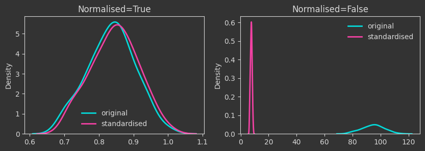
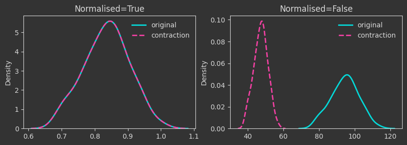
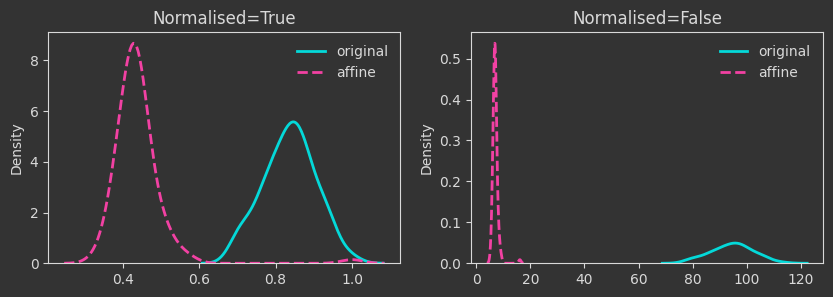
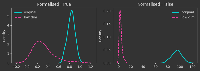
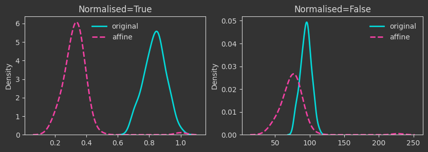
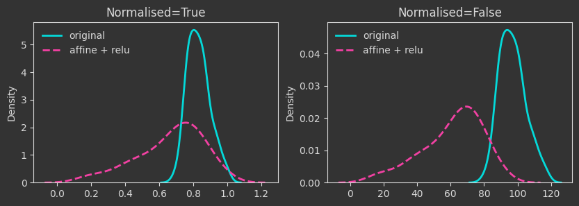
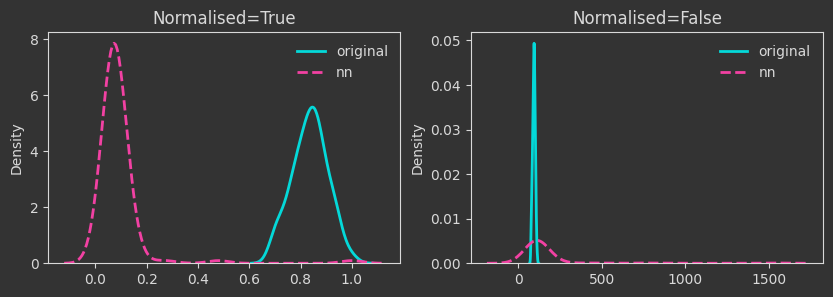
The densities below are kernel-density-estimates (aka., probability densities) of the “death times” of the \(H_0\) homology for the \(X\) point cloud (the one created with make_classification below). But what does “death time” mean here?

Persistent homology (PH) is all about understanding the aspects of the shape of a manifold from sampled points (aka, a point cloud). In this note, we are looking at only one attribute that is captured by PH, the connected components of the manifold. PH looks at the point cloud at various scales, from the scale of the individual points to the scale of the entire dataset. As PH works through the different scales, it identifies when connected components get created (birth) and when they merge (death, for some of them). As every point on its own initially constitutes a connected component, the birth times are all equal to zero.

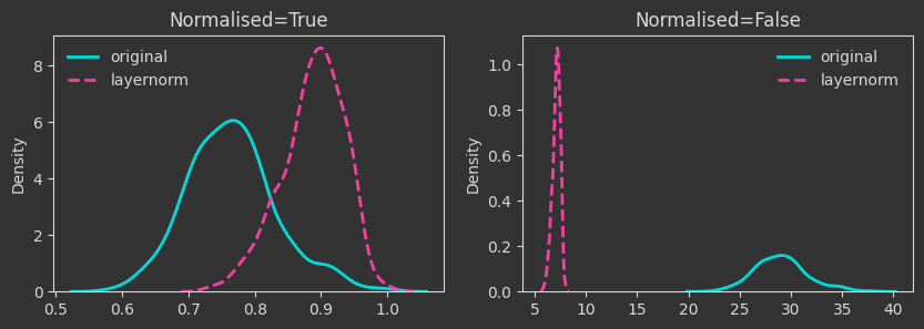
The density plots below are tracking the death times and how those change as we manipulate the point cloud. For each case, I’m showing both the death times as they are (Normalised=False) and what happens if we normalise by the maximum finite persistence time. Normalising them makes the death times invariant to point cloud scaling (as you will see below).

The plots

N_FEAT = 50
X, _ = datasets.make_classification(
    n_classes=2,
    n_samples=100,
    n_features=N_FEAT,
    n_redundant=0,
    n_informative=N_FEAT,
    random_state= 0,
    n_clusters_per_class=4,
    class_sep=1.0
)

# change X to have mean 2 and std 3
X = 2 + 3 * X

# contraction mapping
Xcontr = X / 2

# expansion mapping
Xexp = X * 2

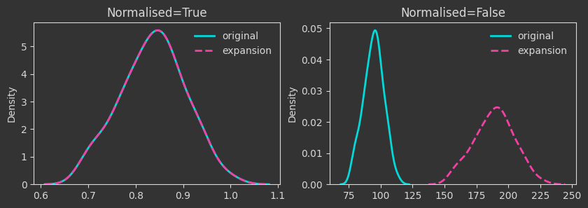
Things are as expected up to this point. A few more interesting operations follow.

# generate a random affine contraction matrix A
A = np.random.rand(N_FEAT, N_FEAT)
A = A  / (np.linalg.norm(A)+1e-10)
b = np.random.rand(N_FEAT)

Xaff = X @ A + b

# map to a lower dimension
Xlow = X[:, :2]

# map to lower dimensions with a random affine map
A = np.random.rand(N_FEAT, 10)
b = np.random.rand(10)


Xaff = X @ A + b

# same affine transformation but with a relu function applied to the output

Xaff_relu = np.maximum(0, X @ A + b)

# two layer neural network with relu activation
N_OUTPUT = 10

A1 = np.random.rand(N_FEAT, 20)
b1 = np.random.rand(20)
A2 = np.random.rand(20, N_OUTPUT)
b2 = np.random.rand(N_OUTPUT)

Xnn = X @ A1 + b1
Xnn = np.maximum(0, Xnn)
Xnn = Xnn @ A2 + b2

# layernorm

Xlayernorm = (X - X.mean(axis=1, keepdims=True)) / X.std(axis=1, keepdims=True)